Speculative decoding combines two things I love: clever systems optimizations and probability. As a result, we have a lot to get through. Lets dig in!
Background: the problem
Suppose you want to run an LLM interactively on your local machine. You have a single GPU, say a GTX 4090. It’s a high-end card, costing $1600, but it’s much cheaper than an A100 or H100 might be. What challenges do you face?
First, the model may not fit on your GPU. Llama2-70B would require 140GB stored in 16-bit precision, 6x larger than what can fit on your device. This problem can be solved by using a smaller model, opting for lower precision through quantization, or both. You compromise and load a 30B parameter model in 4-bit precision. This requires 15GB of storage, leaving you with ample space.
However, you discover that, despite being able to fit your model, it runs at a glacial pace. Huggingface transformers can generate only a few tokens per second at best. Sometimes, it doesn’t even achieve that. You search online for optimized implementations and come across something like exllama that is written in C++ and CUDA. By switching to this well-written optimized code, you find the throughput is closer to 50 tokens per second. That’s an order of magnitude improvement without any change in hardware!
This observation gets you thinking. Surely, 50 tokens per second isn’t the limit, right? There must be a way to achieve faster speeds. Reflecting on the process, you realize that your input prompt processes through the model at a stunning rate, 60x faster than token generation. Mathematically, the prompt undergoes the same procedure as the generated tokens, yet for some reason, one is nearly two orders of magnitude faster than the other. Why is this the case? Both algorithms show 100% utilization on nvidia-smi!
We’ll dive into speculative decoding shortly. But first, let’s delve into GPU Architecture!
From the architecture whitepaper, your RTX4090 looks like this under the hood:

Fig 1. Architecture diagram of RTX 4090.
Zooming in on those streaming multiprocessors (SM), we observe the following structure:

Fig 2. Zoomed in diagram of the streaming multiprocessor (SM).
What does this all mean? And what does it have to do with the generation being so slow? Lets go over all the acronyms in these two pictures:
The processing hierarchy, from top to bottom:
- An NVIDIA GPU is split into various GPU Processing Clusters (GPCs). An RTX4090 has 7.
- A GPC is split into various streaming multiprocessors (SMs). An RTX4090 has 128 SMs, sixteen per GPC.
- An SM is split into four processing blocks. On an RTX4090, each SM has four processing blocks.
The job hierarchy, from bottom to top:
- A thread is an individual unit of work. It executes computation in serial.
- 32 threads are organized in a warp. All threads in a warp run at the same time on the same SM and processing block. An SM can have up to 64 warps scheduled.
- Several warps are organized in a thread block. All threads in a thread block are guaranteed to run on the same SM, but not necessarily at the same time. A thread block can have up to 1024 threads, or 32 warps.
- Thread blocks can (optionally, and only on very recent hardware) be organized into thread block clusters, which run on the same GPU Processing Cluster.
The memory hierarchy, from bottom to top (IMPORTANT):
- Registers / L0 cache - holds per thread or warp. The L0 cache also contains information on which warp is currently running, an SM can have up to 64 warps queued but can only run 4 at a time. One per processing block.
- L1 / shared memory[^1] - this holds information shared between all threads in a thread block. It is quite small (128KB / SM, or 16MB across all SMs), but very fast. Can be explicitly accessed. One per SM
- L2 - 72 MB (in this case) of shared cache. Shared between many SMs and GPCs. Some GPUs have one L2 cache, while some have multiple.
- Main memory - 24GB of memory. Incredibly slow to access versus L0/L1, and much slower than L2
Misc., from most relevant to least:
- Tensor cores do the sweet sweet number crunching used in matmuls. They can only do matrix multiplications of block sizes of blocks eight to sixteen on a side. There is one per SM.
- The CUDA Cores (labeled FP32/Int32 on the diagram) do most of the standard operations outside of matmuls, such as addition, multiplication, etc. They can work on any size, and are roughly an order of magnitude slower than the tensor cores.
- The SFU handles "special" functions, like log, sin, and sqrt
- The RT core does ray tracing. Ignore for now.
- TPC, PolyMorph, and Tex are all pure texture/graphics related. Ignore for now.
For the curious, all that nvidia-smi measures is how often a kernel is executing on the GPU. Any kernel on any part of the GPU would show up as GPU utilization. Adding two vectors together in shared memory on a single SM can achieve 100% utilization for the entire GPU based on nvidia-smi, purely because at every clock step one kernel is executing one step.
This is why something can be insanely slow and still show 100% nvidia-smi usage!
Why did we go into GPU Architecture?
GPU architecture explains precisely why there is a slowdown between processing input prompts (also training) and generation!
(TLDR) On small-batch auto-regressive generation for LLMs, GPUs waste compute cycles on moving the model weights instead of actually computing the output!
To understand why, let's consider the first part of the MLP in a single layer of our transformer. Running the feedforward linear layer on our GPU requires executing several operations. Given a weight matrix \( W \) (defined as \( d_{\mathsf{model}} \times d_{\mathsf{ff}} \)) and an input \( X \) (defined as \( n \times d_{\mathsf{model}} \)), we produce an output \( Y \) (defined as \( n \times d_{\mathsf{ff}} \)) in the following manner:
- Divide the problem into several thread blocks.
- For each thread block, read the relevant submatrix in \( W \) and \( X \) into shared memory.
- Compute the relevant submatrix of \( Y \) and store it in shared memory[a].
- Write this submatrix to the main memory.
At the very minimum, our operations will consist of:
- \( d_{\mathsf{model}} d_{\mathsf{ff}} + nd_{\mathsf{model}} + nd_{\mathsf{ff}} \) reads and writes transitioning from main memory to shared memory.[b]
- \( nd_{\mathsf{model}}d_{\mathsf{ff}} \) floating point operations, commonly referred to as flops.
For the llama2 30B model, where \( d_{\mathsf{model}} = 6656 \) and \( d_{\mathsf{ff}} = 17920 \), and given a prompt of 1024 tokens, we calculate:
\( 2 \times (1024 \times 6656 + 1024 \times 17920 + 6656 \times 17920) = 274 \)MB in 16-bit reads and writes, or 110MB when utilizing four-bit weight quantization. Additionally, it necessitates 122GFlops of 16-bit arithmetic.
If we momentarily set aside all complexities and make a series of generalized assumptions, we can estimate the time required for this operation by dividing the first quantity by the GPU's memory bandwidth, and the second value by the GPU's maximum 16-bit throughput. With our GPU's bandwidth being 1TB/sec and its peak 16-bit throughput reaching 330 trillion floating point operations every second, we derive the following approximate times:
- 0.3ms for reads/writes without quantization, or 0.1ms with.
- 0.3ms for computation.[c]
Bearing in mind that this calculation is for a batch of 1024 tokens, this translates to less than a microsecond per individual token. But let's re-evaluate these figures for just one token:
How do we proceed with this? With a tally of 60MB/238MB reads/writes with and without quantization respectively, we have only 120MFlops worth of calculations to perform. The resulting times are:
- 0.25ms for reads and writes when not using quantization, or 0.05ms with it.
- 0.3 microseconds (or .0003ms) for computation. Given the inability to utilize tensor cores, a more accurate figure might be 0.003ms.
To our surprise, we find that the performance is almost three orders of magnitude slower on a per-token basis! We are spending more time reading and writing than actually making calculations.
- [a] Note that I'm glossing over a ton of detail in how you divide the problem.
- [b] The division of the problem as well as the details of reads and writes are ignored in this post, but have a massive impact. You can't actually achieve this level of efficiency in reads and writes easily in practice. Note, for example, that in this case the size of the reads and writes exceeds the size of the L1/L2 cache without quantization.
- [c] Do you add or take the maximum of these numbers? The answer is complicated. Ideally, we use computation to hide communication, but this rarely works out perfectly in practice.
So… speculative decoding?
What if we made generation more like prefill? How would we do this? We need our model to process more than one token at once. However, to process a token, we need to know that it is part of our output, which we are trying to determine in the first place!
We can’t generate multiple tokens simultaneously without violating joint distribution assumptions1. To achieve accurate and faithful generation, we need to guess. To do this, we employ an ancient method of problem-solving: guess and check.
The model we use to guess can vary. In Blockwise Parallel Decoding for Deep Autoregressive Models, different heads on the same model predicts multiple future tokens (fine-tuned to do so), and the original head checks them. This approach still suffers from the joint distribution problem1. Alternatively, we could perform autoregressive decoding on a smaller model.
It’s important to note that strictly more computation (floating-point operations) is done with speculative decoding, yet we can achieve higher generation throughput. The reason it still saves time is that loading the weights of the small model is much cheaper than the large one, and each token you correctly guess for the future saves an entire load of the model.
Speculative decoding is simply a method to guess in a systematic way using a smaller LLM and to check in a manner that ensures our outputs are identical to using the original. This is what happens in Fast Inference from Transformers via Speculative Decoding and Accelerating Large Language Model Decoding with Speculative Sampling. This may remind you of rejection sampling; we generate candidates using the smaller model and employ the larger model to decide whether we want to accept or reject the sample. We will get into the details shortly.
The final piece of this narrative is the mathematics that makes the outputs of this process identical to the original. Many naive algorithms accidentally oversample outputs that are more common in the smaller model, as they will be guessed by the smaller model more frequently. If you aren’t concerned about exact replication, you can achieve slightly faster results, which is what Speculative Decoding with Big Little Decoder does.
Probability time
For a detailed explanation, refer to the original paper. A brief summary is provided below.
Let \( p(x) \) be the large model's probability distribution, and \( q(x) \) represent the smaller model's distribution. We'll be employing a variation of rejection sampling.
- Sample \( n \) tokens from \( q(x) \), called \( x_1 ... x_n \).
- Generate the logits of the \( n \) tokens from \( p(x) \)
- For each token \( x_i \), decide whether to accept it based on the following criteria:
- If \( q(x_i) < p(x_i) \), accept and move to the next token
- Otherwise, sample a random number \( r \) from \( [0,1] \) and compare it to some value \( v \). We calculate \( v \) as \( \frac{p(x_i)}{q(x_i)} \).
- If it is less than \( v \) , accept anyways
- If it was greater than \( v \), reject, break the loop, and sample the current token from the distribution \( p(x)-q(x) \) where it is positive, normalized to be a probability distribution.
There are several levels of rigor to prove that this algorithm works. We now detail the most intuitive, albeit hand-wavy, explanation:
Assuming \( q(x_i) > p(x_i) \), the probability that our system selects token \( x_i \) is given by \( q(x_i) \cdot \frac{p(x_i)}{q(x_i)} = p(x_i) \). When \( q(x_i) < p(x_i) \), the probability that our system selects the token is \( q(x_i) \) from the initial sampling, plus \( \frac{p(x_i)-q(x_i)}{C} \) from the resampling, where \( C \) is a normalization constant. It can be proven that \( C \) is one because the probabilities across all options must sum to one.
A more rigorous proof is available in the paper, where the distribution specified in step 5 is calculated, along with the probability of any token being sampled from this distribution. The normalization constant is also derived, and the distribution is computed.
In practice, we can leverage the probability distributions of the two models to estimate the number of tokens the smaller model is likely to predict. From the above explanations, the acceptance probability can be calculated as:
- Define \( D \) as a distance metric: \( D(p,q) = \sum_x |\frac{p(x) - q(x)}{2}| = 1-\sum_x \min(p(x), q(x)) \). This is a symmetric divergence for those interested.
- The acceptance probability \( \beta \) for a specific token \( x_i \) is \( \frac{p(x_i)}{q(x_i)} \) if \( q(x_i)>p(x_i) \) and 1 otherwise. This can also be represented as \( \min(1, \frac{p(x_i)}{q(x_i)})=\frac{\min(p(x_i),q(x_i))}{q(x_i)} \).
- We sample from \( q(x) \), hence the general acceptance probability \( \alpha = E(\beta) = \sum_x q(x) \frac{\min(p(x),q(x))}{q(x)} =1-E(D(p,q)) \).
If \( \gamma \) is the number of tokens predicted by the smaller model, then the expected throughput of tokens per iteration for the large model, given an arbitrary acceptance probability \( \alpha \), is visualized in the following figure:
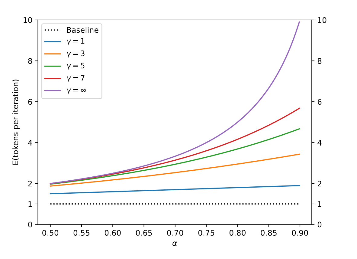
Not bad! However, in the context of this paper and others, \( \alpha \) often hovers around 0.6 to 0.7. The acceptance probability depends on not only how accurate the smaller model is but also its relative generation speed compared to the larger model. In the worst case scenario where the smaller model fails to predict beyond a single token at every iteration, speculative decoding would run slower than not having it in the first place! For LLMs, most works rely on using smaller network from the same model/data family. In the paper we just discussed one would use T5-XXL with T5-BASE/LARGE or LAMDA (137B) with LAMDA (2~8B), something usually in the order of magnitude smaller (in more modern model lingo terms, using LLama2-70B for the bigger model and Llama2-7B as the smaller one). Then the compute break down would look something this:

Fig 3. Simplified transfomer trace diagram. Figure 5. from `Fast Inference from Transformers via Speculative Decoding '.
In summary, smaller model is typically much tinier than the original, making its guessing speed negligible compared to the larger model's checking process. The performance speed up is proprtionate to the small model's ability to approximate the larger one.
But... we still aren't even close!
Using speculative decoding, even with an excellent approximation, we won't generate more than 3-5 tokens per iteration, denoted as \( \gamma \) previously. This might result in a potential 3x speedup at best, which is still short from bridging the theoretical performance gap that is in the orders of magnitude larger.
Efforts have been made to bridge this gap. The paper "Accelerating LLM Inference with Staged Speculative Decoding" introduces two main innovations:
- Employing multiple levels of speculative decoding.
- Generating multiple branched predictions simultaneously.
The latter is somewhat challenging due to nuances in KV caching. The paper doesn't disclose their acceptance probability, and their outcomes are modest. Their method increase the speedup from 2.5x to 3x, but at the expense of introducing substantial complexity.
Personally, I believe there's significant potential yet to be unlocked in this domain. If I were to speculate on the sources of future advancements, I'd anticipate the following:
- Early stopping or AlBERT-style strategies: If the logits of the smaller model could expedite the final decoding.
- This could be further enhanced using distillation.
- One might also adopt aggressive staging, performing only the essential computation needed to reject a proposal.
- Adoption of techniques like Paged Attention to explore multiple branches efficiently at once.
- Implementing structured pruning in tandem with distillation when designing the smaller model. This approach might yield efficient models boasting higher acceptance probabilities.
Conclusion
This post is close to 3000 words, when blog posts are usually kept to the smaller side of a thousand. Congratulations on reading this far, and I hoped you learned something!
-
Imagine you are playing a guessing game with an LLM of the city you grew up in. Given that you are reading this article, it gives a 30% probability of the bay area, and 20% of new york city. If you were generating multiple tokens at once, you might say that for the first token, new and san have 20/30% probability, and for the second york and fran_ have 20/30% probability. A sampling algorithm might pick san york city or even new francity, which are impossible. ↩︎